Train models for the encoder and decoder

This example illustrates the steps required to train and save models for the NDS encoder and decoder. The encoder model is used to convert velocity into spiking rates, while the decoder model is used to predict velocity from spiking rates.

The models will be trained using a slice of data from the dataset Structure and variability of delay activity in premotor cortex and paper with the same title, specifically the data from Session 4 with the subject JenkinsC.

We mostly followed Decoding arm speed during reaching for modeling. One reason to follow this paper specifically is that we wanted to use a model that incorporated the magnitude of the velocity as well as its direction. Traditional cosine tuning curves only include direction.

Download data

Retrieve the preprocessed training data from AWS S3 and validate its checksum.

from urllib.parse import urljoin

import pooch

DOWNLOAD_BASE_URL = "https://neural-data-simulator.s3.amazonaws.com/sample_data/v1/"

BEHAVIOR_DATA_PATH = pooch.retrieve(
    url=urljoin(DOWNLOAD_BASE_URL, "session_4_behavior.npz"),
    known_hash="md5:fff727f5793f62c0bf52e5cf13a96214",
)

SPIKES_TRAIN_DATA_PATH = pooch.retrieve(
    url=urljoin(DOWNLOAD_BASE_URL, "session_4_spikes_train.npz"),
    known_hash="md5:6ba47e77c3045c1d4eda71f892a5cdc3",
)

SPIKES_TEST_DATA_PATH = pooch.retrieve(
    url=urljoin(DOWNLOAD_BASE_URL, "session_4_spikes_test.npz"),
    known_hash="md5:9df38539d794f91049ddc23cc5e04531",
)

Load data

Load the training and test data from the downloaded files.

import matplotlib.pyplot as plt
import numpy as np

behavior_data = np.load(BEHAVIOR_DATA_PATH)
spikes_train_data = np.load(SPIKES_TRAIN_DATA_PATH)
spikes_test_data = np.load(SPIKES_TEST_DATA_PATH)

timestamps = behavior_data["timestamps_train"]
vel_train = behavior_data["vel_train"]
vel_test = behavior_data["vel_test"]
spikes_train = spikes_train_data["spikes_train"]
spikes_test = spikes_test_data["spikes_test"]

assert vel_train.shape[0] == spikes_train.shape[0]

plt.plot(timestamps, vel_train)
plt.xlabel("Time (s)")
plt.show()

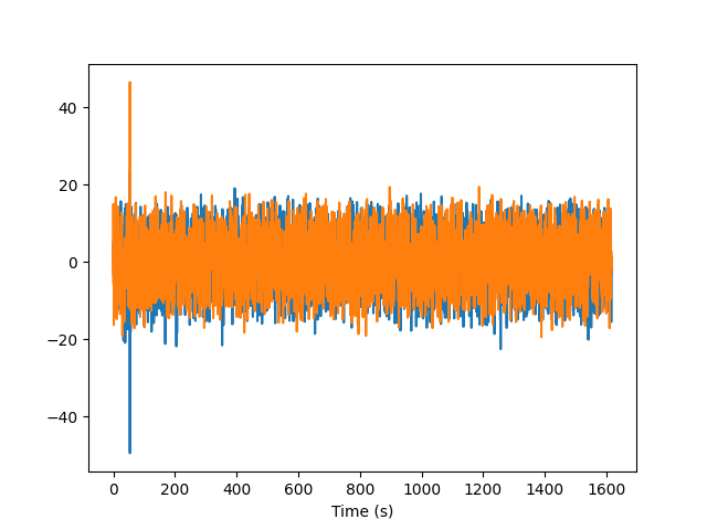
Remove outliers

We observe that at least one sample is an outlier, so let’s remove all outliers from the dataset before training the model.

def get_indices_without_outliers(data, n=9):
    std_dev = np.std(data)
    mean = np.mean(data)
    return np.where(np.any(abs(data - mean) < n * std_dev, axis=1))


vel_train_without_outliers_indices = get_indices_without_outliers(vel_train)
vel_train = vel_train[vel_train_without_outliers_indices]
spikes_train = spikes_train[vel_train_without_outliers_indices]
timestamps = timestamps[vel_train_without_outliers_indices]

assert vel_train.shape[0] == spikes_train.shape[0]

plt.plot(timestamps, vel_train)
plt.xlabel("Time [s]")
plt.show()

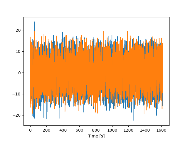
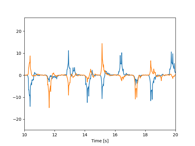
Zoom in on a few trials

Let’s take a look at a few trials to get a better sense of the data.

plt.plot(timestamps, vel_train)
plt.xlabel("Time [s]")
plt.xlim(10, 20)
plt.show()

Standardize velocity

Standardize velocity horizontal and vertical directions by scaling to unit variance.

from sklearn.preprocessing import StandardScaler

scaler = StandardScaler()
scaler.fit(vel_train)

vel_train = scaler.transform(vel_train)
vel_test = scaler.transform(vel_test)

print("scale =", scaler.scale_)
print("mean =", scaler.mean_)
print("var =", scaler.var_)

plt.plot(timestamps, vel_train)
plt.xlabel("Time [s]")
plt.show()

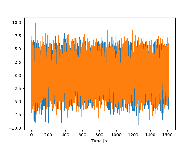
scale = [2.39072966 2.27921963]
mean = [ 0.00231087 -0.01231422]
var = [5.71558832 5.19484214]

Export standardized model for streaming

For replaying the data with the NDS streamer, keep all samples from the dataset, but clip them, then apply the scaler.

import os

from neural_data_simulator.util.runtime import get_sample_data_dir

STANDARDIZED_BEHAVIOR_DATA_PATH = os.path.join(
    get_sample_data_dir(), "session_4_behavior_standardized.npz"
)
VELOCITY_LIMIT = 20

str_timestamps = behavior_data["timestamps_train"]
str_vel_train = np.clip(behavior_data["vel_train"], -VELOCITY_LIMIT, VELOCITY_LIMIT)
str_vel_train = scaler.transform(str_vel_train)
str_vel_test = np.clip(behavior_data["vel_test"], -VELOCITY_LIMIT, VELOCITY_LIMIT)
str_vel_test = scaler.transform(str_vel_test)

np.savez(
    STANDARDIZED_BEHAVIOR_DATA_PATH,
    timestamps_train=str_timestamps,
    vel_train=str_vel_train,
    vel_test=str_vel_test,
)

Create tuning curves

We’re ready to start creating the encoder model. We’ll follow the equation from Decoding arm speed during reaching:

\(spike rate = b_0 + m * |v| * cos(\theta - \theta_{pd}) + b_s*|v|\)

where spike rate is the spike data for the unit we’re trying to model, \(b_0\), \(m\), \(\theta_{pd}\), and \(b_s\) are the coefficients we’re fitting \(\theta_{pd}\) is the preferred direction for this unit, \(\theta\) is the direction of the velocity and \(|v|\) is the magnitude of the velocity.

Note

There is a time delay component removed from the original equation. In the paper, the authors searched for the optimal time delay for each unit. It’s expected that we’ll see spikes happening before the actual movement. For decoding kinematics from spikes, that’s a helpful delay, because you have extra time to process the current spikes as the motor action is only coming in a few milliseconds; but in our case, this means we’d need to use data from the future – or in practice, we’d need to add an extra delay between input and output, which is not desired. So for this initial model, we’ll use “current” behavior data to create “current” spikes.

Let’s fit one model for each unit.

from scipy.optimize import curve_fit


def tuning_model(x, b0, m, pd, bs):
    """
    Spiking rate tuning curve from the paper decoding arm speed during reaching
    """
    mag_vel = np.linalg.norm(x, axis=1)
    theta = np.arctan2(x[:, 1], x[:, 0])
    return b0 + m * mag_vel * np.cos(theta - pd) + bs * mag_vel


class UnitModel:
    """
    Stores key data and model for each unit in our simulation
    """

    def __init__(self, tuning_model, unit_id):
        self.id = unit_id
        self.model_params = []
        self.model_error = []
        self.model = tuning_model

        self.spike_rates_to_fit = None
        self.velocity_to_fit = None

    def fit(self, velocity, spike_rates):
        """
        Find model parameters to spike rates to the velocity using the tuning model
        """
        self.model_params, _ = curve_fit(self.model, velocity, spike_rates)
        self.spike_rates_to_fit = spike_rates
        self.velocity_to_fit = velocity

    def evaluate(self, velocity):
        """
        Get rates based on model fit in the fit function to the given velocities
        """
        rates = self.model(velocity, *self.model_params)
        rates[rates <= 0] = 1e-9
        return rates


units = []
for unit_id in range(spikes_train.shape[1]):
    unit_model = UnitModel(tuning_model, unit_id)
    unit_model.fit(vel_train, spikes_train[:, unit_id])
    units.append(unit_model)

params = np.array([u.model_params for u in units])

Get spiking data from models

In this section, we’ll follow a nomenclature similar to that from the NLB challenge, where rates are the expected number of spikes in a bin – this is what we get out of our original equation when we create our tuning curve model.

simulated_rates_train = np.zeros_like(spikes_train)
for i, u in enumerate(units):
    simulated_rates_train[:, i] = u.evaluate(vel_train)

simulated_rates_test = np.zeros_like(spikes_test)
for i, u in enumerate(units):
    simulated_rates_test[:, i] = u.evaluate(vel_test)

Let’s take a look at what our simulated data looks like compared to the original smoothed binned spiking data to a few randomly chosen units.

from scipy import signal

np.random.seed(20230111)

BIN_WIDTH = 0.02
RANGE_TO_PLOT = slice(2000, 3000)


def smooth_spike_counts(X, *, bin_ms=5, sd_ms=40):
    """
    Smooth the spike counts using a Gaussian filter
    """
    kern_sd = int(round(sd_ms / bin_ms))
    window = signal.gaussian(kern_sd * 6, kern_sd, sym=True)
    window /= np.sum(window)
    filt = lambda x: np.convolve(x, window, "same")
    return np.apply_along_axis(filt, 1, X)


units_to_plot = np.random.choice(np.arange(len(units)), 16)

plt.figure(figsize=(15, 10))
num_rows = 4
num_cols = 4
for i, u in enumerate(units_to_plot):
    plt.subplot(num_rows, num_cols, i + 1)

    # we need to smooth the data after sampling from the poisson
    ys = smooth_spike_counts(
        simulated_rates_train[:, u].reshape(1, -1),
        bin_ms=BIN_WIDTH,
        sd_ms=3 * BIN_WIDTH,
    )
    rel_time = np.arange(RANGE_TO_PLOT.stop - RANGE_TO_PLOT.start) * BIN_WIDTH
    plt.plot(rel_time, ys[0, RANGE_TO_PLOT], label="Simulated (rates)")
    plt.plot(rel_time, spikes_train[RANGE_TO_PLOT, u], alpha=0.5, label="Original")

    # plot y-labels only on left column
    if i % num_cols == 0:
        plt.ylabel("Rates (spk/sec)")
    # plot x-labels only on bottom row
    if i >= num_cols * (num_rows - 1):
        plt.xlabel("Relative time (s)")
# plot legend only on last plot
plt.legend()
plt.show()

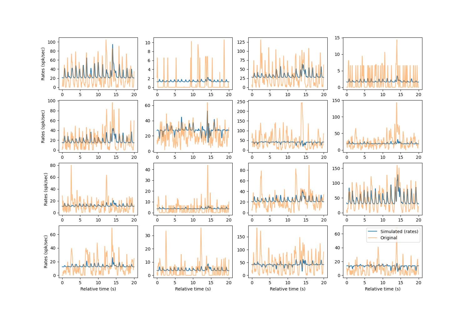
We see that the baseline for each of the rates is nonzero, which is the spiking rate when no movement is being performed.

Evaluate results

To get an idea of how our simulated data is performing, let’s use the evaluation tools from the NLB challenge.

For more information about these metrics, take a look at the NLB challenge evaluation page or at their paper Neural Latents Benchmark ‘21: Evaluating latent variable models of neural population activity.

Cobps

Co-smoothing (cobps) was the main metric used for the challenge which is based on the log-likelihood of neurons activity. cobps would be 0 if the predicted rates were the average of the actual spike rate. The higher cobps the better.

It’s hard to interpret cobps though, as you can’t infer from the cobps results from other datasets. Here, we calculate a few different cobps for this dataset to try to get a better sense of how well we’re doing. However, this will be more useful as we create new models as this will allow us to tell whether our models are improving.

from nlb_tools.evaluation import bits_per_spike

r = simulated_rates_train.reshape(
    1, simulated_rates_train.shape[0], simulated_rates_train.shape[1]
)
s = spikes_train.reshape(1, spikes_train.shape[0], spikes_train.shape[1])

print(f"cobps for original data (i.e. best achievable): {bits_per_spike(s, s)}")
print(
    "cobps for mean per channel (this should be 0 by the co-bps definition): "
    f"{bits_per_spike(np.ones_like(s)*np.mean(s, axis=1), s)}"
)
print(
    "cobps for mean across all training data: "
    f"{bits_per_spike(np.ones_like(s)*np.mean(s), s)}"
)
print(
    "cobps for random uniform data: "
    f"{bits_per_spike(np.random.uniform(np.min(s), np.max(s), size=s.shape), s)}"
)
print(f"cobps for simulated data (train data): {bits_per_spike(r, s)}")

r = simulated_rates_test.reshape(
    1, simulated_rates_test.shape[0], simulated_rates_test.shape[1]
)
s = spikes_test.reshape(1, spikes_test.shape[0], spikes_test.shape[1])
print(f"cobps for simulated data (test data): {bits_per_spike(r, s)}")

neg_log_likelihood: Zero rate predictions found. Replacing zeros with 1e-9
cobps for original data (i.e. best achievable): 0.44869971234258726
cobps for mean per channel (this should be 0 by the co-bps definition): 0.0
cobps for mean across all training data: -0.48506622301885116
cobps for random uniform data: -9.126104175688969
cobps for simulated data (train data): 0.02553927440612118
cobps for simulated data (test data): 0.01976954526713931

\(R^2\) of behavioral data

Another way that the quality of generated spikes was evaluated for the NLB challenge was using them on ridge regression model trained with actual data.

Here we’ll do a similar approach, but we’ll try different combinations of training/testing with real or simulated data to try to extract more information.

from nlb_tools.evaluation import fit_and_eval_decoder

r2 = fit_and_eval_decoder(spikes_train, vel_train, spikes_test, vel_test)
print(f"trained on real data, tested on real data: {r2}")
r2 = fit_and_eval_decoder(spikes_train, vel_train, simulated_rates_test, vel_test)
print(f"trained on real data, tested on simulated data: {r2}")
r2 = fit_and_eval_decoder(simulated_rates_train, vel_train, spikes_test, vel_test)
print(f"trained on simulated data, tested on real data: {r2}")
r2 = fit_and_eval_decoder(
    simulated_rates_train, vel_train, simulated_rates_test, vel_test
)
print(f"trained on simulated data, tested on simulated data: {r2}")

trained on real data, tested on real data: 0.4935748125484304
trained on real data, tested on simulated data: 0.7756907188111652
trained on simulated data, tested on real data: -1.114126355973245
trained on simulated data, tested on simulated data: 0.9999999999999726

Export the encoder model to a file

Save the velocity tuning curve parameters to a file that can be used in the encoder configuration.

ENCODER_MODEL_PATH = os.path.join(
    get_sample_data_dir(), "session_4_tuning_curves_params.npz"
)

params = np.array([u.model_params for u in units])

np.savez(
    ENCODER_MODEL_PATH,
    b0=params[:, 0],
    m=params[:, 1],
    pd=params[:, 2],
    bs=params[:, 3],
)

Train a model for the decoder

Fit a model to predict velocity from the spiking data.

from sklearn.linear_model import Ridge

decoder = Ridge()
decoder.fit(spikes_train, vel_train)
real_score = decoder.score(spikes_test, vel_test)
sim_score = decoder.score(simulated_rates_test, vel_test)

print(f"trained on real data, tested on real spikes: {real_score}")
print(f"trained on real data, tested on simulated spikes: {sim_score}")

trained on real data, tested on real spikes: 0.4935748125484304
trained on real data, tested on simulated spikes: 0.7756907188111652

Export the decoder model to a file

Dump the model to a file that can be used in the decoder configuration.

import joblib

DECODER_MODEL_PATH = os.path.join(
    get_sample_data_dir(), "session_4_simple_decoder.joblib"
)

joblib.dump(decoder, DECODER_MODEL_PATH)

['/home/runner/.nds/sample_data/session_4_simple_decoder.joblib']