Visualize the input behavior together with the decoded behavior

The goal of this example is to display the input behavior aligned with the decoded behavior in a plot.

By default, this script will download the data to be plotted from AWS S3. If you prefer to use your own data, you can start the closed loop simulation in one terminal:

make run-closed-loop

And then record the streams in another terminal:

recorder --session "decode_example" --lsl "NDS-Behavior,NDS-Decoder" --recording-time 10

Make sure to change the variable:

LOCAL_DATA = True

and replace the variable with the path to your data:

BEHAVIOR_DATA_PATH = "the_path_to_your_recorded_behavior_data.npz"
DECODER_DATA_PATH = "the_path_to_your_recorded_decoder_data.npz"

Environment setup

LOCAL_DATA = False

Set data source

Retrieve the data from AWS S3 or define the path to your local file.

from urllib.parse import urljoin

import pooch

DOWNLOAD_BASE_URL = "https://neural-data-simulator.s3.amazonaws.com/sample_data/v1/"

if not LOCAL_DATA:
    BEHAVIOR_DATA_PATH = pooch.retrieve(
        url=urljoin(DOWNLOAD_BASE_URL, "decode_example_NDS-Behavior.npz"),
        known_hash="md5:201cbd92f432b94ce8dcb8fb87c07634",
    )

    DECODER_DATA_PATH = pooch.retrieve(
        url=urljoin(DOWNLOAD_BASE_URL, "decode_example_NDS-Decoder.npz"),
        known_hash="md5:a6a59c08dc32819a6781383e0ba1b4c1",
    )

else:
    BEHAVIOR_DATA_PATH = "the_path_to_your_recorded_behavior_data.npz"
    DECODER_DATA_PATH = "the_path_to_your_recorded_decoder_data.npz"

Load data

Load the data to be plotted.

import matplotlib.pyplot as plt
import numpy as np
from scipy import signal
from sklearn.metrics import r2_score

behavior_file = np.load(BEHAVIOR_DATA_PATH)
behavior_data = behavior_file["data"]
behavior_timestamps = behavior_file["timestamps"] - behavior_file["timestamps"][0]

decoder_file = np.load(DECODER_DATA_PATH)
decoder_data = decoder_file["data"]
decoder_timestamps = decoder_file["timestamps"] - decoder_file["timestamps"][0]

Plot data

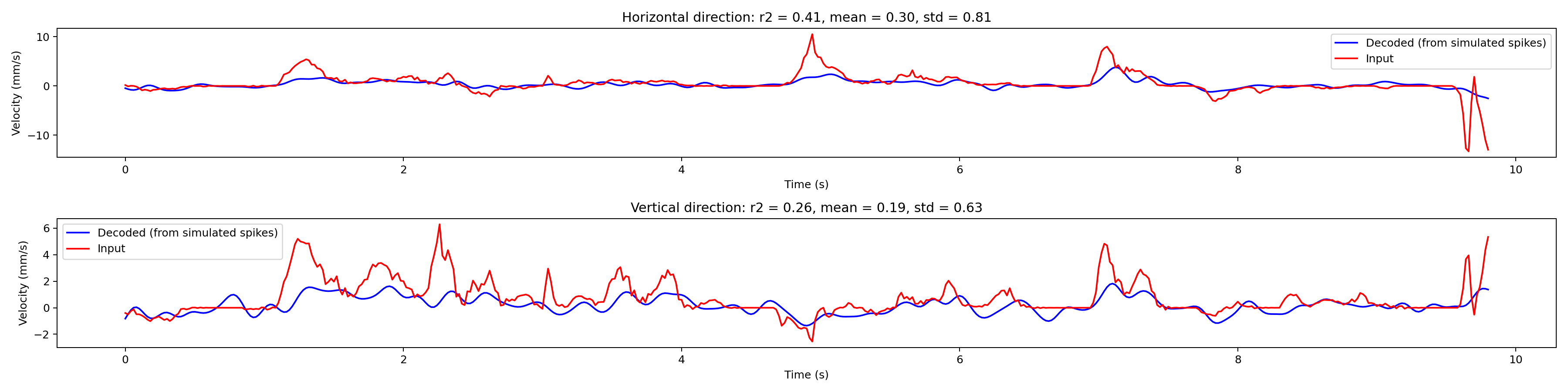
def _plot_velocities(
    behavior_data: np.ndarray,
    behavior_timestamps: np.ndarray,
    decoder_data: np.ndarray,
    r2: np.ndarray,
    axis: int,
):
    mean = np.mean(decoder_data[:, axis])
    std = np.std(decoder_data[:, axis])
    if axis == 0:
        plt.title(
            (
                f"Horizontal direction: r2 = {r2[axis]:.2f}, "
                f"mean = {mean:.2f}, std = {std:.2f}"
            )
        )
    else:
        plt.title(
            (
                f"Vertical direction: r2 = {r2[axis]:.2f}, "
                f"mean = {mean:.2f}, std = {std:.2f}"
            )
        )

    plt.plot(
        behavior_timestamps,
        decoder_data[:, axis],
        "blue",
        label="Decoded (from simulated spikes)",
    )
    plt.plot(
        behavior_timestamps,
        behavior_data[:, axis],
        "red",
        label="Input",
    )
    plt.ylabel("Velocity (mm/s)")
    plt.xlabel("Time (s)")
    plt.legend()


def get_lag(x: np.ndarray, y: np.ndarray):
    correlation = signal.correlate(x, y, mode="full")
    lags = signal.correlation_lags(x.size, y.size, mode="full")
    lag = lags[np.argmax(correlation)]
    return abs(lag)


h_lag = get_lag(behavior_data[:, 0], decoder_data[:, 0])

behavior_data = behavior_data[:, :]
behavior_timestamps = np.array(behavior_timestamps)[:]
behavior_timestamps = behavior_timestamps - behavior_timestamps[0]
decoder_data = decoder_data[h_lag:, :]

# cut behavior and decoder streams to the same length
min_samples = min(decoder_data.shape[0], behavior_data.shape[0])
decoder_data = decoder_data[:min_samples, :]
behavior_data = behavior_data[:min_samples, :]
behavior_timestamps = behavior_timestamps[:min_samples]

r2 = r2_score(behavior_data, decoder_data, multioutput="raw_values")

dpi = 180
fig_size = (20, 5)
plt.figure(num="Velocities overview", dpi=dpi, figsize=fig_size)

plt.subplot(2, 1, 1)
_plot_velocities(behavior_data, behavior_timestamps, decoder_data, r2, axis=0)

plt.subplot(2, 1, 2)
_plot_velocities(behavior_data, behavior_timestamps, decoder_data, r2, axis=1)

plt.tight_layout()
plt.show()