Visualize spike rates for input behavior

The goal of this example is to show the spike rates predicted by the encoder for a given behavior input.

By default, this script will download the data to be plotted from AWS S3. If you prefer to use your own data, you can start the closed loop simulation in one terminal:

make run-closed-loop

And then record the streams in another terminal:

recorder --session "test" --lsl "NDS-Behavior,NDS-SpikeRates,NDS-RawData" --recording-time 10

Make sure to change the variable:

LOCAL_DATA = True

and replace the variables with the paths to your data:

BEHAVIOR_DATA_PATH = "the_path_to_your_recorded_behavior_data.npz"
SPIKES_RATES_DATA_PATH = "the_path_to_your_recorded_spikes_rate_data.npz"
RAW_DATA_PATH = "the_path_to_your_recorded_raw_data.npz"

Environment setup

WITH_RAW_DATA = False
LOCAL_DATA = False

Set data source

Retrieve the data from AWS S3 or define the path to your local files.

from urllib.parse import urljoin

import pooch

DOWNLOAD_BASE_URL = "https://neural-data-simulator.s3.amazonaws.com/sample_data/v1/"

if not LOCAL_DATA:
    BEHAVIOR_DATA_PATH = pooch.retrieve(
        url=urljoin(DOWNLOAD_BASE_URL, "example_NDS-Behavior.npz"),
        known_hash="md5:5c95928f48a71eb3370885c58e14e765",
    )
    SPIKES_RATES_DATA_PATH = pooch.retrieve(
        url=urljoin(DOWNLOAD_BASE_URL, "example_NDS-SpikeRates.npz"),
        known_hash="md5:64fe24f817969afb6d330283a78bca5f",
    )
    if WITH_RAW_DATA:
        RAW_DATA_PATH = pooch.retrieve(
            url=urljoin(DOWNLOAD_BASE_URL, "example_NDS-RawData.npz"),
            known_hash="md5:887d88387674d8a7d27726e11663eee4",
        )
else:
    BEHAVIOR_DATA_PATH = "the_path_to_your_recorded_behavior_data.npz"
    SPIKES_RATES_DATA_PATH = "the_path_to_your_recorded_spikes_rate_data.npz"
    RAW_DATA_PATH = "the_path_to_your_recorded_raw_data.npz"

Load data

Load the data to be plotted.

from matplotlib.pyplot import figure
import matplotlib.pyplot as plt
import numpy as np

behavior_file = np.load(BEHAVIOR_DATA_PATH)
spike_rates_file = np.load(SPIKES_RATES_DATA_PATH)

spike_rates_data = spike_rates_file["data"]
spike_rates_timestamps = (
    spike_rates_file["timestamps"] - spike_rates_file["timestamps"][0]
)

behavior_data = behavior_file["data"]
behavior_timestamps = behavior_file["timestamps"] - behavior_file["timestamps"][0]

if WITH_RAW_DATA:
    raw_file = np.load(RAW_DATA_PATH)
    raw_data = raw_file["data"] / 4
    raw_timestamps = raw_file["timestamps"] - raw_file["timestamps"][0]

Plot data

plt.rcParams.update({"font.size": 14})

figure(figsize=(20, 5), dpi=180)
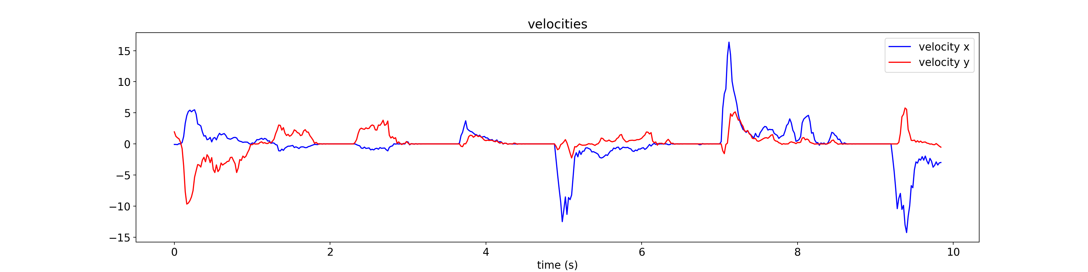
plt.plot(behavior_timestamps, behavior_data[:, 0], "blue", label="velocity x")
plt.plot(behavior_timestamps, behavior_data[:, 1], "red", label="velocity y")

plt.xlabel("time (s)")
plt.legend()
plt.title("velocities")
plt.show()


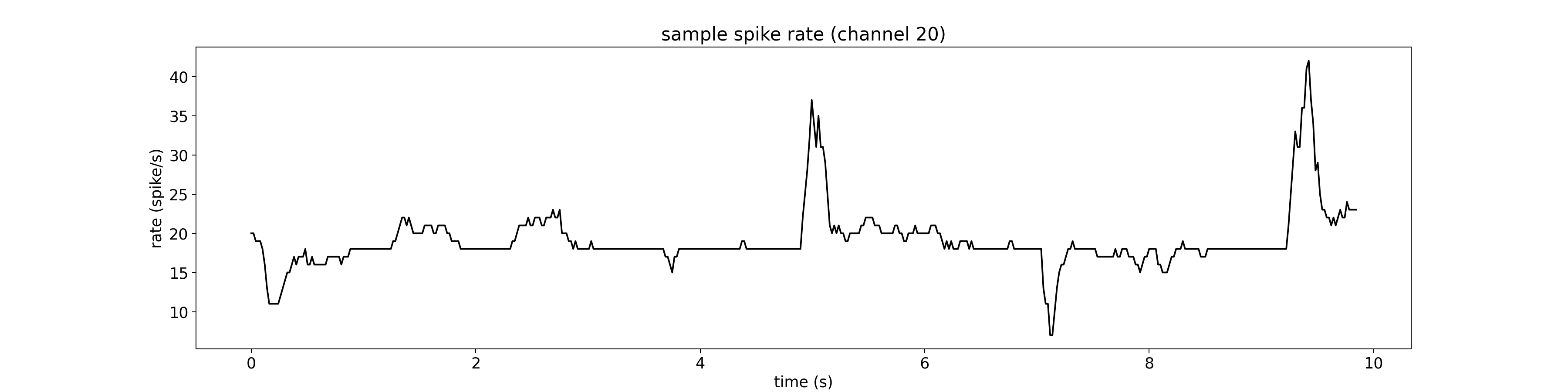
figure(figsize=(20, 5), dpi=180)
plt.plot(
    spike_rates_timestamps,
    spike_rates_data[:, 20],
    "k",
    label="Spike rates",
    linewidth=1.5,
)

plt.ylabel("rate (spike/s)")
plt.xlabel("time (s)")
plt.title("sample spike rate (channel 20)")
plt.show()

if WITH_RAW_DATA:
    figure(figsize=(20, 5), dpi=180)
    plt.plot(raw_timestamps, raw_data[:, 20], "k", label="Raw data", alpha=0.8)
    plt.ylabel("signal amplitude (uV)")
    plt.xlabel("time (s)")
    plt.title("sample raw output (channel 20)")
    plt.show()

• 
•