Chapter 6

Analyzing Neural Time Series Data

Python code for Chapter 6 – converted from original Matlab by AE Studio (and ChatGPT)
Original Matlab code by Mike X Cohen

This code accompanies the book, titled “Analyzing Neural Time Series Data” (MIT Press).
Using the code without following the book may lead to confusion, incorrect data analyses, and misinterpretations of results.
Mike X Cohen and AE Studio assume no responsibility for inappropriate or incorrect use of this code.

Import necessary libraries

import numpy as np
import matplotlib.pyplot as plt

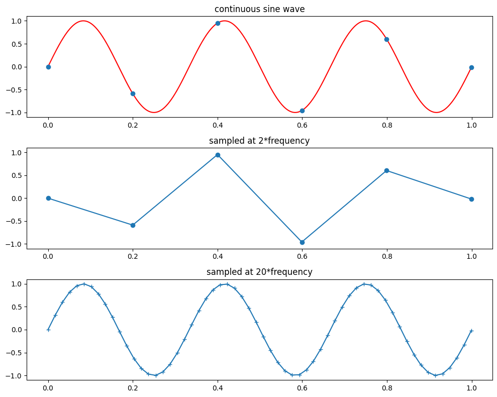
Figure 6.2

# Create sine wave
srate = 1000
time = np.arange(0, 1, 1/srate)
frequency = 3

sinewave = np.sin(2 * np.pi * frequency * time)

# Plot the continuous sine wave and sampled sine waves
plt.figure(figsize=(10, 8))

# Continuous sine wave
plt.subplot(311)
plt.plot(time, sinewave, 'r')
plt.xlim([-.05, time[-1] * 1.05])
plt.ylim([-1.1, 1.1])
plt.title('continuous sine wave')
sampling1 = np.round(np.linspace(0, len(time)-1, frequency*2)).astype(int)
plt.plot(time[sampling1], sinewave[sampling1], 'o')

# Sampled at 2*frequency
plt.subplot(312)
plt.plot(time[sampling1], sinewave[sampling1], '-o')
plt.xlim([-.05, time[-1] * 1.05])
plt.ylim([-1.1, 1.1])
plt.title('sampled at 2*frequency')

# Sampled at 20*frequency
sampling2 = np.round(np.linspace(0, len(time)-1, frequency*20)).astype(int)
plt.subplot(313)
plt.plot(time[sampling2], sinewave[sampling2], '-+')
plt.title('sampled at 20*frequency')
plt.xlim([-.05, time[-1] * 1.05])
plt.ylim([-1.1, 1.1])

plt.tight_layout()
plt.show()